Heat Transfer Euler Method Continuous Functions and Field Theory

We considered one such representation already: the climate. This can be thought of as a continuous function

          [temperature, pressure, humidity, wind velocity(3)] =           Weather (longitude,latitude,elevation,time)        

The state is thus a 6-tuple of continuous variables, each of which depends on 4 continuous parameters. The governing equations are partial differential equations (PDEs), which describes how each of the 6 variables changes as a function of all the others. Other, simpler examples include

Heat flow (Temperature(position,time))

Diffusion (Concentration(position,time))

Electrostatic or Gravitational potential (Potential(position))

Electromagnetic field strength (Field(position,time))

Fluid flow (Velocity,Pressure,Density(position,time))

Semiconductor modeling (Electron_density(position,time))

Quantum Mechanics (Wave_function(position,time))

Elasticity (Stress,Strain(position,time))

We will derive the heat equation in some detail, and later show that the computational bottleneck is identical to that for electrostatic or gravitational potential.

Consider a long thin bar of length one, of uniform material, and insulated so that heat can enter or escape only at its ends. Let u(x,t) be the temperature at position 0 <= x <= 1, and time t >= 0. Consider a short stretch of bar between x and x+h. It is a fact one can measure in the laboratory, that the rate H(x) at which heat flows from x to x+h is proportional to the temperature gradient (u(x,t)-u(x+h,t))/h. (H(x)>0, so heat flows from x to x+h, if u(x,t) > u(x+h,t).) H(x-h)-H(x) is the rate at which heat flows toward x, from both x-h and x+h, and so is the rate at which heat "builds up" at x. Dividing (H(x-h)-H(x)) by h yields the rate at which the "heat density" builds up at x, which is in turn proportional to the rate at which the temperature rises or falls at x. In other words

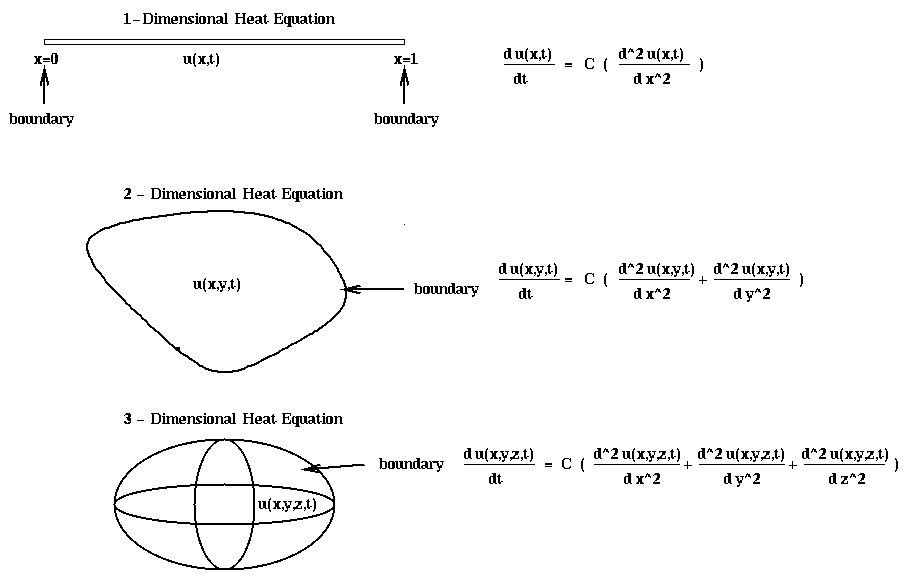
          d u(x,t)       (u(x-h,t)-u(x,t))/h - (u(x,t)-u(x+h,t))/h         -------- = C * -----------------------------------------            dt                              h        

where C is a constant of proportionality. For small h,

          u(x-h,t)-u(x,t)        d u( x - h/2, t)          ---------------   ~  - ----------------                 h                      dt    and          u(x,t)-u(x+h,t)        d u( x + h/2, t)          ---------------   ~  - ----------------                 h                      dt    and so          (u(x-h,t)-u(x,t))/h - (u(x,t)-u(x+h,t))/h      d^2 u(x,t)          -----------------------------------------  ~  ----------                              h                             d x^2        

Thus in the limit as h --> 0, we get the heat equation

          d u(x,t)       d^2 u(x,t)           -------- = C * ----------              dt             d x^2        

C is called the conductivity of the bar. To solve this equation, we still need the boundary conditions, or the temperatures at the ends of the bar (u(0,t) and u(1,t) for all t >= 0), and the initial conditions, or the temperature of the bar at time t=0 (u(x,0) for all 0 <= x <= 1).

If instead of a 1-dimensional bar, we have a 2-dimensional plate of some shape, the heat equation becomes

          d u(x,y,t)         d^2 u(x,y,t)   d^2 u(x,y,t)           ---------- = C * ( ------------ + ------------ )               dt                 d x^2          d y^2                       = C * 2D-Laplacian(u)        

with boundary conditions consisting of temperature specified all along the 1-dimensional boundary of the plate, and the initial conditions consisting of the temperature at every point in the plate at t=0.

Finally, if we have a complete 3-dimensional object, the heat equation becomes

          d u(x,y,z,t)         d^2 u(x,y,z,t)   d^2 u(x,y,z,t)   d^2 u(x,y,z,t)      ------------ = C * ( -------------- + -------------- + -------------- )           dt                  d x^2            d y^2            d z^2                                    = C * 3D-Laplacian(u)        

with boundary conditions consisting of temperature all along the 2-dimensional boundary of the body, and initial conditions consisting of the temperature throughout the body at t=0. (Note that the Laplacian is defined both for functions of 2 and of 3 variables.)

Let us show how to solve the 1-dimensional heat equation. For simplicity, we take C=1. Since the problem is continuous, we need to discretize it to reduce it to a finite problem we can solve. We will use finite differences to do this, meaning that we will only compute u(x,t) on a computational grid or mesh (x(i),t(m)), where x(i) = i*h, 0 <= i <= n = 1/h, where h is the mesh spacing in the x direction, and t(m) = m*k, where k is the time step. We approximate u(x,t) on this grid by computing it at the grid points u(x(i),t(m)). We denote our approximation at this point by U(i,m), as shown in the figure below.

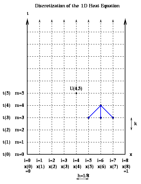
The initial condition u(x,0) tells us the value of U(i,0) at all the grid points along the bottom row in the figure, the boundary condition u(0,t) tells us the value of U(0,m) at the all grid points along the left boundary of the figure, and the boundary condition u(1.0,t) tells us the value of U(n,m) at all the grid points along the right boundary of the figure.

Having discretized the state variable u(x,t), the initial condition, and the boundary conditions, we need to discretize the governing equation. There are a variety of ways to do this. The simplest way is analogous to the forward Euler method we described in the last lecture. We approximate du(x(i)-h/2,t(m))/dx and du(x(i)+h/2,t(m))/dx by the finite differences

d u( x(i)-h/2, t(m) )   u( x(i), t(m) ) - u( x(i)-h, t(m) )   U(i,m)-U(i-1,m) --------------------- ~ ----------------------------------- ~ ---------------         dx                              h                            h  and  d u( x(i)+h/2, t(m) )   u( x(i)+h, t(m) ) - u( x(i), t(m) )   U(i+1,m)-U(i,m) --------------------- ~ ----------------------------------- ~ ---------------         dx                              h                            h        

and then d^2 u(x(i),t(m))/ dx^2 by the finite difference

          d^2 u(x(i),t(m))   d u( x(i)+h/2, t(m) )/dx  -  d u( x(i)-h/2, t(m) )/dx     ---------------- ~ -----------------------------------------------------           d^2 x                                  h                        u(x(i-1),t(m)) - 2*u(x(i),t(m)) + u(x(i+1),t(m))                      ~ ------------------------------------------------                                               h^2                        U(i-1,m) -2*U(i,m) + U(i+1,m)                      ~ -----------------------------                                     h^2        

We then approximate d u(x,t)/dt by

          d u(x(i),t(m))   u(x(i),t(m+1)) - u(x(i),t(m))   U(i,m+1) - U(i,m)     -------------- ~ ----------------------------- ~ -----------------           d t                      k                         k        

Combining the last two expressions yields the equation

          U(i,m+1) - U(i,m)   U(i-1,m) - 2*U(i,m) + U(i+1,m)     ----------------- = ------------------------------              k                       h^2        

To use this as an algorithm, we assume we know the temperature u for all x(i) at time t(m), and solve the equation for the temperature for all x(i) at the next time step t(m+1)=t(m)+k:

          k      U(i,m+1) =  U(i,m) + ( --- ) * ( U(i-1,m) - 2*U(i,m) + U(i+1,m) )                            h^2               =  z * U(i-1,m) + (1-2*z) * U(i,m) + z * U(i+1,m)        

where z = k/h^2 is a constant. In terms of the last figure, this gives us a formula to compute the values of U(i,m+1) at all the internal grid points in row m+1 of the discretization, in terms of the values of U(m,i) in row m.

          Explicit solution of the 1D Heat Equation       for m = 1 to final m          for i = 1 to n-1               U(i,m+1) =  z * U(i-1,m) + (1-2*z) * U(i,m) + z * U(i+1,m)          end for      end for        

The algorithm is called explicit because it uses an explicit formula for the value of U(i,m+1) in terms of old data. Note that U(i,m+1) depends on exactly three values in the row below it. This pattern is indicated in blue in the discretization above, and is called the stencil of the algorithm.

Parallelism is available in this problem by dividing the mesh on the bar up into contiguous pieces, and assigning them to different processors, with processors responsible for updating the values at the mesh points they own. This is shown in the figure below for 4 processors. Since the boundary points require no computation, the leftmost and rightmost processors have 1 fewer grid point to update. Because the stencil only requires data from grid points to the immediate left and right, only data at the boundary of the processors needs to be communicated. Thus, the parallelism shares the surface-to-volume effect with our parallelization of particle systems, because most work is in internal to the data owned by a processor, and only data on the boundary needs to be communicated.

Unfortunately, the restriction k <= .5 h^2 on the time step for the explicit solution of the heat equation means we need to take excessively tiny time steps, even after the solution becomes quite smooth. This makes it expensive to compute the solution at large times. As with stiff ODEs, the correct alternative is to use an implicit method which requires solving a linear system at each step. The simplest reasonable implicit method is called Crank-Nicholson, and uses the discretization

          u(x(i),t(m+1)) - u(x(i),t(m))        ----------------------------- ~                  k                                     1      u(x(i-1),t(m))   - 2*u(x(i),t(m))   + u(x(i+1),t(m))                 - * ( -----------------------------------------------------                 2                         h^2                           u(x(i-1),t(m+1)) - 2*u(x(i),t(m+1)) + u(x(i+1),t(m+1))                    + ------------------------------------------------------)                                         h^2        

leading to the formula

          U(i,m+1) - U(i,m)        ----------------- =              k                                         1      U(i-1,m)   - 2*U(i,m)   + U(i+1,m)                     - * ( -----------------------------------                     2                     h^2                                 U(i-1,m+1) - 2*U(i,m+1) + U(i+1,m+1)                          + ------------------------------------ )                                               h^2        

Solving for U(*,m+1) yields

          -z/2 * U(i-1,m+1) + (1+z) * U(i,m+1) - z/2 * U(i+1,m+1) =                z/2 * U(i-1,m) + (1-z) * U(i,m) + z/2 * U(i+1,m)        

where as before z=k/h^2. This may also be written as a tridiagonal linear system of equations

          [ 1+z    -z/2                     ]   [ U(1,m+1)   ]             [ -z/2   1+z    -z/2              ]   [ U(2,m+1)   ]            [         ...                     ]   [  ...       ]          [        -z/2   1+z   -z/2        ] * [ U(i,m+1)   ] =          [                ...              ]   [  ...       ]           [               -z/2  1+z   -z/2  ]   [ U(n-2,m+1) ]          [                     -z/2  1+z   ]   [ U(n-1,m+1) ]                      [                (1-z) * U(1,m) + z/2 * U(2,m)       ]                     [ z/2 * U(1,m) + (1-z) * U(2,m) + z/2 * U(3,m)       ]                     [                     ...                            ]                     [ z/2 * U(i-1,m) + (1-z) * U(i,m) + z/2 * U(i+1,m)   ]                     [                     ...                            ]                     [ z/2 * U(n-3,m) + (1-z) * U(n-2,m) + z/2 * U(n-1,m) ]                     [ z/2 * U(n-2,m) + (1-z) * U(n-1,m)                  ]        

where for simplicity we have used the boundary conditions U(0,:) = U(n,:) = 0. We may abbreviate this linear system as

          ( I + (z/2)*T) * U(:,m+1) = b(m) = ( I - (z/2)*T) * U(:,m)        

where T is the tridiagonal matrix

          [  2 -1          ]          [ -1  2 -1       ]      T = [     ...        ]          [       -1  2 -1 ]          [          -1  2 ]        

This leads to the overall algorithm

          Implicit solution of the 1D Heat Equation -- Crank-Nicholson       for m = 1 to final m          b(m) = ( I - (z/2)*T) * U(:,m)           Solve ( I+(z/2)*T)*U(:,m+1) = b(m) for U(:,m+1)      end for        

(For a proof that the solution remains bounded no matter how large a time step we take, see

We will look at the 2D heat equation on a square plate. We discretize the plate with a 2D mesh as follows. u(i,j,m) refers to the value of u(x(i),y(j),t(m)) at the mesh point x(i)=i*h, y(j)=j*h, and at time t(m)=m*k. Sometimes we will just write u(i,j) to refer to the value of u(x(i),y(j)) at the mesh point x(i)=i*h, y(j)=j*h.

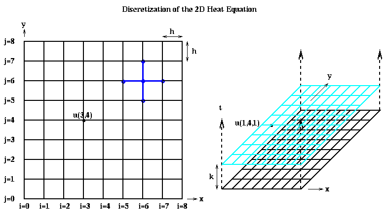
We approximate the two second-derivatives of u with respect to x and y similarly as before:

          d^2 u(x(i),y(j),t(m))        ---------------------            d x^2                                                        u(x(i-1),y(j),t(m)) - 2*u(x(i),y(j),t(m)) + u(x(i+1),y(j),t(m))           ~ ---------------------------------------------------------------                                         h^2              U(i-1,j,m) - 2*U(i,j,m) + U(i+1,j,m)           ~ ------------------------------------                             h^2 and     d^2 u(x(i),y(j),t(m))        ---------------------            d y^2                                                        u(x(i),y(j-1),t(m)) - 2*u(x(i),y(j),t(m)) + u(x(i),y(j+1),t(m))           ~ ---------------------------------------------------------------                                         h^2              U(i,j-1,m) - 2*U(i,j,m) + U(i,j+1,m)           = ------------------------------------                             h^2 so summing the last two terms                           U(i-1,j) + U(i+1,j) + U(i,j-1) + U(i,j+1) - 4*U(i,j)   2D-Laplacian(U)(i,j) ~ ----------------------------------------------------                                                  h^2                         = Discrete-2D-Laplacian(U)(i,j)        

As with the 1D Heat Equation, we can use either the explicit Euler algorithm:

          U(i,j,m+1) - U(i,j,m)       --------------------- = Discrete-2D-Laplacian(U)(i,j)                  k        

which is equivalent to

          U(i,j,m+1) = U(i,j,m) + k*Discrete-2D-Laplacian(U)(i,j,m)                              k                                    = (1 - 4*---) * U(i,j,m) +                             h^2                                     k                     ---*(U(i-1,j,m) + U(i+1,j,m) + U(i,j-1,m) + U(i,j+1,m))                     h^2        

or the implicit Crank-Nicholson algorithm:

          U(i,j,m+1) - U(i,j,m)   1    --------------------- = - * ( Discrete-2D-Laplacian(U)(i,j,m+1) +                k            2                                  Discrete-2D-Laplacian(U)(i,j,m) )        

which is equivalent to

          k    U(i,j,m+1)  -  - * Discrete-2D-Laplacian(U)(i,j,m+1) =                   2                                         k                            U(i,j,m)  +  - * Discrete-2D-Laplacian(U)(i,j,m)                                          2        

or

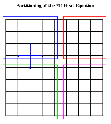
          k                    k    (1 + 2*---) * U(i,j,m+1) - ----- * ( U(i-1,j,m+1) + U(i+1,j,m+1) +            h^2                 2*h^2                                         U(i,j-1,m+1) + U(i,j+1,m+1) )                     k                  k          = (1 - 2*---) * U(i,j,m) + ----- * ( U(i-1,j,m) + U(i+1,j,m) +                    h^2               2*h^2                                               U(i,j-1,m) + U(i,j+1,m) )           = b(i,j,m)        

As before, implementing Euler's method involves setting each U(i,j,m+1) to a weighted average of its north, south, east and west neighbors on a grid; this stencil is shown in blue above and below. Parallelization involves assigning subsets of grid points to processors, as shown below.

Implementing Crank-Nicholson requires solving a system of linear equations. Let us show what this matrix looks like. To write down this matrix, we need to make a linear list of the unknowns U(i,j,m+1), so we can put them in a vector. We illustrate below:

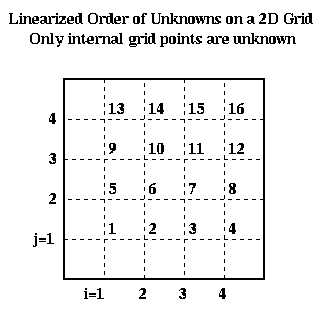
For simplicity, let a = 1+2*k/h^2 and c = -k/(2*h^2). This lets us write the linear system as H*U=b, or

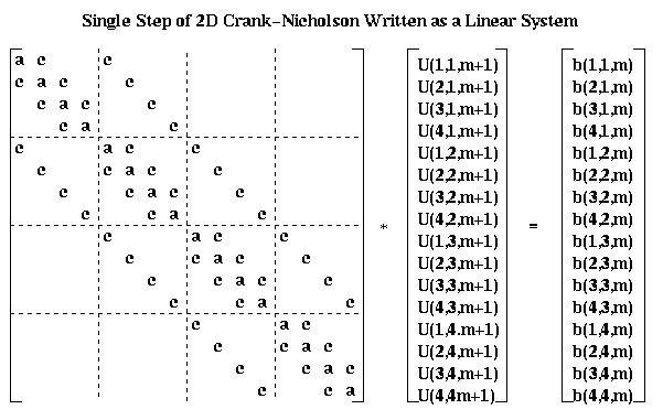
More generally, we get an (n-1)^2-by-(n-1)^2 block-tridiagonal matrix, with blocks that are (n-1)-by-(n-1). The diagonal blocks are identical tridiagonal matrices with a on the diagonal and c on the offdiagonals. The offdiagonal blocks are all c times the (n-1)-by-(n-1) identity matrix.

As just described, we have two algorithms: explicit (Euler) and implicit (Crank-Nicholson). The explicit algorithm is be easy to parallelize, by dividing the physical domain (square plate) into subsets, and having each processor update the grid points on the subset it owns. However, we will be limited to unreasonably tiny time steps to keep the solution stable, so computing the solution for large times will require many steps. The implicit solution will let us take large time steps while retaining stability, but will be much more interesting to parallelize. Because of the ability to take large time steps, and because we can parallelize successfully, the implicit algorithm is the algorithm of choice. Even on a serial machine, the linear system for one step of Crank-Nicholson on the 2D heat equation is a much more interesting linear system to solve than the 1D case, where we had a tridiagonal system. On a serial machine, we can solve a tridiagonal system using band Gaussian elimination (i.e. Gaussian elimination which does not store or do arithmetic with zero entries outside the non zero band) in time proportional to the number of unknowns, i.e. about the same time as the explicit Euler algorithm. The 2D (and analogous 3D) problems are much harder to do efficiently, and a great deal of ingenuity has been spent solving these problems in serial and in parallel. The following is a table of the complexity of solving this system using a number of standard algorithms. N=(n-1)^2 is the number of unknowns (16 in the above example). All quantities are to be interpreted in the O(.) sense. The Serial Time is the time to solve on a serial processor. The PRAM Time is the time to solve on a parallel processors with free communication and #Procs processors (we will have much to say about the true costs of these algorithms, including communication, in later lectures). Storage is the amount of memory required. Type = D means the algorithm is direct, i.e. it gives the exact answer after the indicated number of steps (modulo round off errors). Type = I means the algorithm is iterative, i.e. that it repeatedly updates an approximate solution, so that the solution converges as we do more iterations. The number of iterations required depends on the matrix entries a and b, and the desired accuracy. For this table we have chosen the important special case of a=4 and c=-1.

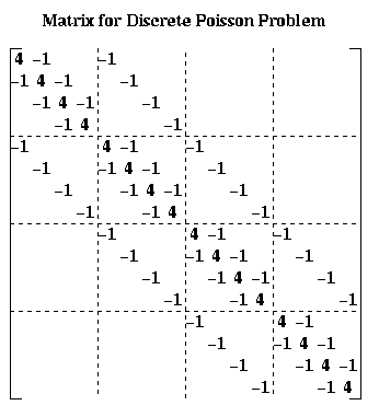
This special case is called the discrete Poisson equation. We call the above matrix H in the discussion below. See the section on electrostatic force and gravity below to see where this case arises. Given these values of a and c, we have chosen the number of iterations so the solution provides about as accurate a solution to the underlying continuous heat equation as the direct methods (i.e. taking the discretization error into account).

            Algorithm   Type  Serial Time     PRAM Time      Storage  #Procs     ---------   ----  -----------     ---------      -------  ------    Dense LU      D       N^3              N           N^2      N^2    Band LU       D       N^2              N         N^(3/2)     N    Jacobi        I       N^2              N            N        N    Inv(H)*b      D       N^2            log N         N^2      N^2    CG            I       N^(3/2)      N^(1/2)*log N    N        N    SOR           I       N^(3/2)      N^(1/2)          N        N    Sparse LU     D       N^(3/2)      N^(1/2)       N*log N     N    FFT           D       N*log N        log N          N        N    Multigrid     I       N              (log N)^2      N        N    Lower Bound           N              log N          N   Key to abbreviations:      Dense LU: Gaussian elimination, treating H as dense      Band LU : Gaussian elimination, treating H as zero outside a band                                      of half-width n-1 near diagonal      Sparse LU : Gaussian elimination, exploiting entire                                         zero-structure of H      Inv(H)*b : precompute and store inverse of H, multiply it by                    right-hand-side b      CG      : Conjugate Gradient method      SOR     : Successive Overrelaxation      FFT     : Fast Fourier Transform based method        

There are several interesting features of this table. The Lower Bound is the time required to compute any N numbers which are themselves nontrivial functions of N other numbers. Note that this lower bound is actually attained (in the O(.) sense) both in the serial and parallel cases, but by different algorithms. Multigrid is the fastest serial algorithm, and the FFT is second fastest. In the PRAM model, they trade places, and the FFT is fastest. Later we will study both algorithms, which use divide-and-conquer but in quite different ways: parallelizing the FFT requires fast matrix transposes, and Multigrid requires operating on a quadtree. In particular, we will do more realistic performance modeling, incorporating communication time, in order to see which one is faster in practice.

We include a variety of other algorithms, not because they are competitive for the discrete Poisson equation, but because they are more widely applicable than to the discrete Poisson equation. Dense LU (Gaussian elimination) is discussed at length in other lectures. Band LU is similar, but avoids storage and arithmetic outside the bandwidth of size sqrt(N)=n-1. Both result in filling in many of the zero entries in the coefficient matrix. Sparse LU exploits the entire zero structure of H (and its L and U factors) to avoid all storage of and arithmetic with 0 entries. It will be discussed in another lecture.

The method inv(H)*b means that we precompute and store the explicit inverse of H once and for all; this is not counted as part of the computational cost, but just storage. Then solving a linear system H*x=b requires multiplying b by the explicit inverse, at a cost of 2n^2 serial flops. This method is impractical because of the enormous storage required, and is not even as fast as the most rudimentary iterative method, Jacobi.

Jacobi's method is an iterative solver, and at each iteration replaces the current approximate solution at (i,j) by a weighted average of its nearest neighbors on the grid; its stencil is the same as for Euler. It therefore is parallelized much like the explicit Euler solver. SOR (Successive Overrelaxation) uses a more clever weighted average than Jacobi, and also only updates the grid points in two phases. It converges much more quickly. Jacobi and SOR work best on matrices, like H, that are diagonally dominant, i.e. where the diagonal is sufficiently larger than the offdiagonals.

CG (Conjugate Gradients) applies to any linear system system like H*x=b, where H is a symmetric matrix as well as positive definite. Such matrices are very common in engineering practice. (Three equivalent definitions of positive definiteness are that (1) all of H's eigenvalues must be positive; (2) x'*H*x > 0 for all nonzero vectors x; and (3) there must be an LU factorization of the form H = L*L'.) The computational bottleneck of CG is a matrix-vector multiplication by H, and so effective parallelization requires grid partitioning as described earlier.

To see why essentially the same PDE as described heat flow also describes gravity and electrostatic force, recall that both of these forces satisfy an inverse square law. This means that the force on a particle at (x,y,z), due to a particle at the origin, is proportional to

          -(x,y,z)/r^3        

where r = sqrt(x^2 + y^2 + z^2). Instead of dealing with the force, which is a vector, it is easier to deal with a potential V(x,y,z), which is the scalar

          V(x,y,z) = -1 / r        

One can easily confirm that the force is just the negative of the gradient of the potential

          d V(x,y,z)   d V(x,y,z)   d V(x,y,z)      - grad V(x,y,z) = - ( ---------- , ---------- , ---------- )                                dx           dy           dz        

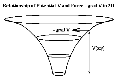
The intuition behind the potential is that V is the height of a hill at a point (x,y,z), and the corresponding force just pushes a particle at (x,y,z) downhill, in the direction of steepest descent (the direction in which V decreases most rapidly). This is shown below in 2D.

It is straightforward to confirm that V(x,y,z) satisfies

          3D-Laplacian(V) = 0        

except at r=0, where V has a singularity. The above equation is called Laplace's equation. When masses or charged particles are present (the more interesting case), then we instead get Poisson's equation

          3D-Laplacian(V) = f        

where f describes the density of mass or of charge. Combined with appropriate boundary conditions (like the value of V along a square boundary), these equations can be solved by discretizing the same way as in the last section. Thus, we may solve for electrostatic or gravitational force by first computing the potential V by solving Poisson's equation numerically, and then computing the gradient of V numerically.

For simplicity we often consider gravity or electrostatic forces in the plane, by which we mean the solution of the 2D problem

          2D-Laplacian(V) = f        

This is not a real physical potential, but captures mathematically many of the properties of the real problem, and since it is 2D and so cheaper to solve than the 3D problem, it is widely used. Discretizing it using the same finite difference approach as above yields the discrete Poisson equation H*v=f, where v is a vector of unknowns, f is given and H is the discrete Poisson matrix described in the last section.

howardtwoubleff.blogspot.com

Source: https://people.eecs.berkeley.edu/~demmel/cs267/lecture17/lecture17.html

Share this post